One-Way ANOVA
Original Author: Kyle R. Ripley
Updated on 6/25/2020 by Kyle R. Ripley
1 Overview
In this tutorial, we’ll cover how to perform a one-way ANOVA using both lm() and aov(), and we’ll see how to create specific contrast codes for use in the analyses. We’ll be using the iris dataset available in R to look at the differences in Sepal.Length of different iris Species.
1.1 Packages (and versions) used in this document
## [1] "R version 4.0.2 (2020-06-22)"## Package Version
## ggplot2 3.3.2
## ggeffects 0.16.0
## car 3.0-9
## lsr 0.5
## compute.es 0.2-5
## multcomp 1.4-13
## pastecs 1.3.212 One-way ANOVA
2.1 Getting Familiar with the Data
Before jumping into the analysis, let’s take a peek at our data. We’ll use str() to check the class of our variables, and we’ll use summary() to get an overview of our data frame - such as missingness, distribution information of variables, etc.
str(iris)## 'data.frame': 150 obs. of 5 variables:
## $ Sepal.Length: num 5.1 4.9 4.7 4.6 5 5.4 4.6 5 4.4 4.9 ...
## $ Sepal.Width : num 3.5 3 3.2 3.1 3.6 3.9 3.4 3.4 2.9 3.1 ...
## $ Petal.Length: num 1.4 1.4 1.3 1.5 1.4 1.7 1.4 1.5 1.4 1.5 ...
## $ Petal.Width : num 0.2 0.2 0.2 0.2 0.2 0.4 0.3 0.2 0.2 0.1 ...
## $ Species : Factor w/ 3 levels "setosa","versicolor",..: 1 1 1 1 1 1 1 1 1 1 ...From the str() output, we can see that our measurement variables are all of the numeric class, and the Species variable is a factor, which is what we want.
summary(iris)## Sepal.Length Sepal.Width Petal.Length Petal.Width
## Min. :4.300 Min. :2.000 Min. :1.000 Min. :0.100
## 1st Qu.:5.100 1st Qu.:2.800 1st Qu.:1.600 1st Qu.:0.300
## Median :5.800 Median :3.000 Median :4.350 Median :1.300
## Mean :5.843 Mean :3.057 Mean :3.758 Mean :1.199
## 3rd Qu.:6.400 3rd Qu.:3.300 3rd Qu.:5.100 3rd Qu.:1.800
## Max. :7.900 Max. :4.400 Max. :6.900 Max. :2.500
## Species
## setosa :50
## versicolor:50
## virginica :50
##
##
## From the summary() output, we can see that we have equal sample sizes in each level of Species. We can also see some distributional information about the measurement variables.
We may also want to get an idea of what our data may look like visually.
ggplot(data = iris, mapping = aes(x = Species, y = Sepal.Length)) +
  geom_line(group = 1, stat = "summary", fun = "mean") +
  geom_point(stat = "summary", fun = "mean") +
  geom_errorbar(stat = "summary", width = 0.2, fun.data = "mean_cl_normal") +
  jtools::theme_apa() +
  labs(x = "Iris Species", y = "Mean Sepal Length")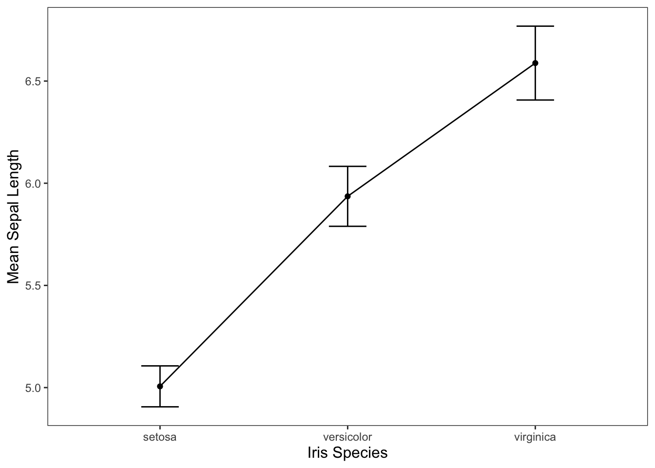
2.1.1 Descriptive Statistics
It’ll also be helpful in reporting our results to have some idea of what our descriptive statistics are. We can use the stat.desc() function from the pastecs package to get the overall descriptive statistics for our variable of interest, Sepal.Length.
stat.desc(iris$Sepal.Length)## nbr.val nbr.null nbr.na min max range
## 150.00000000 0.00000000 0.00000000 4.30000000 7.90000000 3.60000000
## sum median mean SE.mean CI.mean.0.95 var
## 876.50000000 5.80000000 5.84333333 0.06761132 0.13360085 0.68569351
## std.dev coef.var
## 0.82806613 0.14171126We could also combine stat.desc() with by() to specify that we want descriptive statistics for Sepal.Length for each level of Species, as shown below.
by(iris$Sepal.Length, iris$Species, stat.desc)## iris$Species: setosa
## nbr.val nbr.null nbr.na min max range
## 50.00000000 0.00000000 0.00000000 4.30000000 5.80000000 1.50000000
## sum median mean SE.mean CI.mean.0.95 var
## 250.30000000 5.00000000 5.00600000 0.04984957 0.10017646 0.12424898
## std.dev coef.var
## 0.35248969 0.07041344
## ------------------------------------------------------------
## iris$Species: versicolor
## nbr.val nbr.null nbr.na min max range
## 50.00000000 0.00000000 0.00000000 4.90000000 7.00000000 2.10000000
## sum median mean SE.mean CI.mean.0.95 var
## 296.80000000 5.90000000 5.93600000 0.07299762 0.14669422 0.26643265
## std.dev coef.var
## 0.51617115 0.08695606
## ------------------------------------------------------------
## iris$Species: virginica
## nbr.val nbr.null nbr.na min max range
## 50.00000000 0.00000000 0.00000000 4.90000000 7.90000000 3.00000000
## sum median mean SE.mean CI.mean.0.95 var
## 329.40000000 6.50000000 6.58800000 0.08992695 0.18071498 0.40434286
## std.dev coef.var
## 0.63587959 0.096520892.2 The Analysis
We can go about performing this one-way ANOVA a few different ways.
2.2.1 lm()
We could use the lm() function that we discussed in the Simple Linear Regression tutorial. If we use the summary() funciton to examine the output of our model, we’ll get our one-way ANOVA output in the traditional regression format.
m1r <- lm(Sepal.Length ~ Species, data = iris)
summary(m1r)
##
## Call:
## lm(formula = Sepal.Length ~ Species, data = iris)
##
## Residuals:
## Min 1Q Median 3Q Max
## -1.6880 -0.3285 -0.0060 0.3120 1.3120
##
## Coefficients:
## Estimate Std. Error t value Pr(>|t|)
## (Intercept) 5.0060 0.0728 68.762 < 2e-16 ***
## Speciesversicolor 0.9300 0.1030 9.033 8.77e-16 ***
## Speciesvirginica 1.5820 0.1030 15.366 < 2e-16 ***
## ---
## Signif. codes: 0 '***' 0.001 '**' 0.01 '*' 0.05 '.' 0.1 ' ' 1
##
## Residual standard error: 0.5148 on 147 degrees of freedom
## Multiple R-squared: 0.6187, Adjusted R-squared: 0.6135
## F-statistic: 119.3 on 2 and 147 DF, p-value: < 2.2e-16Notice that the above output gives you the means of your groups as the estimates. The intercept is the mean of the reference group (setosa in this case), and the estimates for versicolor and virginica are the differences between those groups and the reference group.
We can get our output in the typicall ANOVA omnibus fashion by using the anova() function instead. This output will tell us if there are significant differences between the levels of Species (which we saw in the previous summary()).
anova(m1r)## Analysis of Variance Table
##
## Response: Sepal.Length
## Df Sum Sq Mean Sq F value Pr(>F)
## Species 2 63.212 31.606 119.26 < 2.2e-16 ***
## Residuals 147 38.956 0.265
## ---
## Signif. codes: 0 '***' 0.001 '**' 0.01 '*' 0.05 '.' 0.1 ' ' 12.2.2 aov()
Instead of lm(), we could choose to use the aov() function. This function performs very similarly to lm() because it is a wrapper around the lm() function. Basically, this means that aov() is just a special case of lm() with slightly different defaults. The main difference that you’ll see if that when we use summary() with aov() (as shown below), we get the traditional ANOVA omnibus output.
m1a <- aov(Sepal.Length ~ Species, data = iris)
summary(m1a)
## Df Sum Sq Mean Sq F value Pr(>F)
## Species 2 63.21 31.606 119.3 <2e-16 ***
## Residuals 147 38.96 0.265
## ---
## Signif. codes: 0 '***' 0.001 '**' 0.01 '*' 0.05 '.' 0.1 ' ' 1If you wish, you can still get the regression-style output by using summary.lm().
summary.lm(m1a)##
## Call:
## aov(formula = Sepal.Length ~ Species, data = iris)
##
## Residuals:
## Min 1Q Median 3Q Max
## -1.6880 -0.3285 -0.0060 0.3120 1.3120
##
## Coefficients:
## Estimate Std. Error t value Pr(>|t|)
## (Intercept) 5.0060 0.0728 68.762 < 2e-16 ***
## Speciesversicolor 0.9300 0.1030 9.033 8.77e-16 ***
## Speciesvirginica 1.5820 0.1030 15.366 < 2e-16 ***
## ---
## Signif. codes: 0 '***' 0.001 '**' 0.01 '*' 0.05 '.' 0.1 ' ' 1
##
## Residual standard error: 0.5148 on 147 degrees of freedom
## Multiple R-squared: 0.6187, Adjusted R-squared: 0.6135
## F-statistic: 119.3 on 2 and 147 DF, p-value: < 2.2e-16We could also get a measure of \(\eta^2\) using the etaSquared() function.
etaSquared(m1a, anova = TRUE)## eta.sq eta.sq.part SS df MS F p
## Species 0.6187057 0.6187057 63.21213 2 31.6060667 119.2645 0
## Residuals 0.3812943 NA 38.95620 147 0.2650082 NA NA2.2.3 Contrast Codes
It’s important to note that lm() and aov() default to using a dummy coding scheme for comparisons. This is fine for some purposes, but you may also wish to use a different set of contrast codes. We’ll look at how to do that in this section.
levels(iris$Species)## [1] "setosa" "versicolor" "virginica"We have three different levels of Species. We can ask n-1 different questions about the variable, so we can make 3-1=2 different contrast codes. For our first contrast code, let’s say that we’re interested in if setosa is significantly different than versicolor. We can look at the levels(iris$Species) output above to refresh ourselves on what order the levels are.
contrast1 <- c(-1, 1, 0)For our second contrast code, let’s look to see if versicolor and virginica are significantly different from each other.
contrast2 <- c(0, 1, -1)Now that we have our contrast codes made, we need to apply them to our Species variable.
contrasts(iris$Species) <- cbind(contrast1, contrast2)We can double check that we did our contrast codes correctly by using the contrasts() function.
contrasts(iris$Species)## contrast1 contrast2
## setosa -1 0
## versicolor 1 1
## virginica 0 -1Let’s go ahead and run our one-way ANOVA with our new contrast codes.
m2a <- aov(Sepal.Length ~ Species, data = iris)
summary(m2a)
## Df Sum Sq Mean Sq F value Pr(>F)
## Species 2 63.21 31.606 119.3 <2e-16 ***
## Residuals 147 38.96 0.265
## ---
## Signif. codes: 0 '***' 0.001 '**' 0.01 '*' 0.05 '.' 0.1 ' ' 1Notice that the omnibus ANOVA output doesn’t change - this is to be expected. We’ll see the difference when we look at the regression output with summary.lm()
summary.lm(m2a)##
## Call:
## aov(formula = Sepal.Length ~ Species, data = iris)
##
## Residuals:
## Min 1Q Median 3Q Max
## -1.6880 -0.3285 -0.0060 0.3120 1.3120
##
## Coefficients:
## Estimate Std. Error t value Pr(>|t|)
## (Intercept) 5.84333 0.04203 139.02 <2e-16 ***
## Speciescontrast1 0.83733 0.05944 14.09 <2e-16 ***
## Speciescontrast2 -0.74467 0.05944 -12.53 <2e-16 ***
## ---
## Signif. codes: 0 '***' 0.001 '**' 0.01 '*' 0.05 '.' 0.1 ' ' 1
##
## Residual standard error: 0.5148 on 147 degrees of freedom
## Multiple R-squared: 0.6187, Adjusted R-squared: 0.6135
## F-statistic: 119.3 on 2 and 147 DF, p-value: < 2.2e-162.3 Visualizing the Results
Often, you’ll see the results of one-way ANOVAs visualized through bar graphs. We can use the code below to do that for the iris data. If you need a refresher on visualizing data in R, check out the Graphing in ggplot2 tutorial.
ggplot(data = iris, mapping = aes(x = Species, y = Sepal.Length)) +
  geom_bar(stat = "summary", fun = "mean") +
  geom_errorbar(stat = "summary", width = 0.2, fun.data = "mean_cl_normal") +
  jtools::theme_apa() +
  labs(x = "Iris Species", y = "Mean Sepal Length")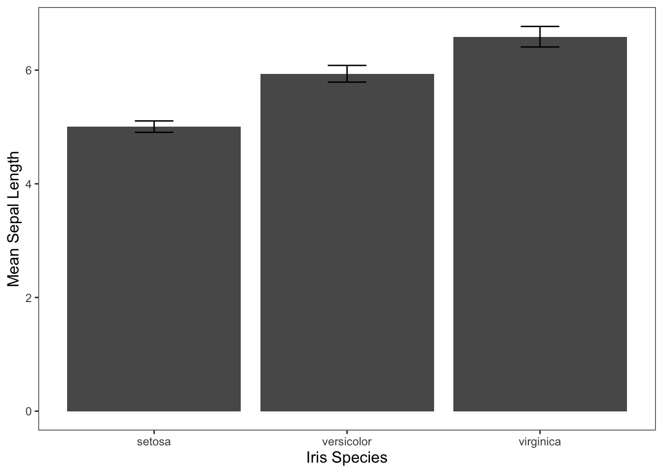
We could also use the line graph that we created earlier (provided below), but be careful doing this. Using a line graph tends to imply some level of continuity in your categorical variables even if there isn’t any.
ggplot(data = iris, mapping = aes(x = Species, y = Sepal.Length)) +
  geom_line(group = 1, stat = "summary", fun = "mean") +
  geom_point(stat = "summary", fun = "mean") +
  geom_errorbar(stat = "summary", width = 0.2, fun.data = "mean_cl_normal") +
  jtools::theme_apa() +
  labs(x = "Iris Species", y = "Mean Sepal Length")