Simple Linear Regression
Original Author: Kyle R. Ripley
Updated on 6/25/2020 by Kyle R. Ripley
1 Overview
In this tutorial, we’ll cover how to perform a simple linear regression step by step. We’ll then look at how to do it quicker and easier using the lm() function in R. We’ll also look at some easy ways to perform diagnostics for our regression analysis. For this tutorial, we’ll be using the cars dataset available in R to predict stopping distances (dist) of cars based on their speed before stopping.
1.1 Packages (and versions) used in this document
## [1] "R version 4.0.2 (2020-06-22)"## Package Version
## ggplot2 3.3.2
## olsrr 0.5.32 Step by Step Regression
Before we get started, let’s take a little peek at the data. In this data frame, we have two variables, speed and dist.
head(cars)## speed dist
## 1 4 2
## 2 4 10
## 3 7 4
## 4 7 22
## 5 8 16
## 6 9 102.1 Compact Model
Our first step for conducting the regression ‘by hand’ is to create our compact model. This is a model that will attempt to predict our outcome variable, dist, using no additional parameters other than the mean of dist. We can express this model in equation form: \[Y_i=\beta_0+\epsilon_i \]
Let’s go ahead and calculate that mean and assign it to mean_dist.
(mean_dist <- mean(cars$dist))## [1] 42.98Now that we have mean_dist, we can calculate the error for our compact model, error_c, by subtracting mean_dist from the original dist variable.
cars$error_c <- cars$dist - mean_distWe then need to square these values to get our squared error of our compact model, sq_error_c.
cars$sq_error_c <- cars$error_c^2Now that we have sq_error_c we can simply add those values together to get our sum of squared error of our compact model, sse_c.`
(sse_c <- sum(cars$sq_error_c))## [1] 32538.982.2 Augmented Model
Next, we’ll begin working on our augmented model. This model will contain all of the parameters from our compact model in addition to any parameters we wish to add to the model. We only have one other variable in our data frame that we can use as a parameter, speed, so let’s write out that equation and then calculate our mean_speed. \[Y_i=\beta_0+\beta_1X_{i1}+\epsilon_i \]
(mean_speed <- mean(cars$speed))## [1] 15.4Now that we have mean_speed, we can begin calculating the slope of our speed variable. First we need to calculate the individual differences between each observation of speed and mean_speed. We’ll then use this vector to calculate the numerator and denominator of our slope formula.
cars$x_diff <- cars$speed - mean_speedLet’s take our differences, x_diff, and multiply them by our error from the compact model, error_c. We’ll then add these values together to get our slope numerator.
(slope_num <- sum(cars$x_diff * cars$error_c))## [1] 5387.4To calculate our slop denominator, we need to square x_diff and then sum the values.
(slope_denom <- sum(cars$x_diff^2))## [1] 1370We now have both of the required elements to calculate our slope value. We’ll simply divide slope_num by slope_denom.
(slope <- slope_num/slope_denom)## [1] 3.932409Because we now know the value of our speed variable’s slope, we can calculate the intercept value by subtracting the product of the slope of speed and mean_speed from the mean of distance, mean_dist.
(intercept <- mean_dist - slope * mean_speed)## [1] -17.57909From here, we can begin calculating the sum of squared error for our augmented model. The first step will be to calculate the dist values that our model will predict given the slope and intercept values we calculated.
cars$pred_a <- intercept + slope * cars$speedWe can then calculate the error between our predicted values, pred_a, and the actual distance values.
cars$error_a <- cars$dist - cars$pred_aNow we’ll square those values…
cars$sq_error_a <- cars$error_a^2…and sum them to get our sum of squared error for our augmented model, sse_a.
(sse_a <- sum(cars$sq_error_a))## [1] 11353.522.3 Proportional Reduction in Error
We’ll now calculate the proportional reduction in error (PRE) which represents the proportion of error from the compact model that is reduced or eliminated when we use the more complex augmented model.
(pre <- 1 - (sse_a/sse_c))## [1] 0.6510794We can see that adding the speed predictor to the model reduced the error by 65%.
We can then use the pre value to calculate our F-value. We’ll start off by calculating the numerator of F by dividing pre by the difference in number of parameters between the augmented and compact models.
(f_num <- pre/(2-1)) # parameters in aug - params in comp## [1] 0.6510794Next, we’ll calculate the denominator of F using pre. The denominator of the below formula represents the sample size (n) and the number of parameters in the augmented model.
(f_denom <- (1 - pre)/(length(cars$dist) - 2)) # n - param in aug## [1] 0.00726918Finally, we can calculate F by dividing f_num by f_denom.
(f_stat <- f_num/f_denom)## [1] 89.56711We can also calculate our t-value by taking the square root of f_stat.
(t_stat <- sqrt(f_stat))## [1] 9.463993 Regression Using lm()
Doing a simple regression following the above steps is useful for understanding how the values are derived, but it isn’t very practical for everyday use. Below, we’ll look at how to quickly conduct a regression analysis in R using the lm() function.
To start, lm() uses a formula to specify the analysis that you’re wanting to conduct. Simply put, these analyses are formatted outcome variable ~ predictor variable. If you’re looking to use multiple predictor variables, give the Multiple Regression tutorial a read through. In that tutorial, we’ll cover how to specify multiple predictors.
The lm() function has many potential arguments that we won’t use in this analysis, so if you have any questions about using lm() that aren’t answered here, you can always run ?lm in your console to bring up the documentation for the function.
In the below code, you can see that we’re wanting to predict dist from speed.
mod_a <- lm(dist ~ speed, data = cars)We ran our model, but to see the results of the analysis, we need to use the summary() function.
summary(mod_a)##
## Call:
## lm(formula = dist ~ speed, data = cars)
##
## Residuals:
## Min 1Q Median 3Q Max
## -29.069 -9.525 -2.272 9.215 43.201
##
## Coefficients:
## Estimate Std. Error t value Pr(>|t|)
## (Intercept) -17.5791 6.7584 -2.601 0.0123 *
## speed 3.9324 0.4155 9.464 1.49e-12 ***
## ---
## Signif. codes: 0 '***' 0.001 '**' 0.01 '*' 0.05 '.' 0.1 ' ' 1
##
## Residual standard error: 15.38 on 48 degrees of freedom
## Multiple R-squared: 0.6511, Adjusted R-squared: 0.6438
## F-statistic: 89.57 on 1 and 48 DF, p-value: 1.49e-12Think back to the values that we calculated earlier. Do they match the values shown in the summary output?
They’re the same! Additionally, we can see that the PRE value is reported as Multiple R-squared.
You may also want to calculate confidence intervals around your predictor. This is easy to do with the confint() function. You just need to supply the object you want confidence intervals for (our model, mod_a) and the level (such as 90%, 95%, etc.).
confint(object = mod_a, level = 0.95)## 2.5 % 97.5 %
## (Intercept) -31.167850 -3.990340
## speed 3.096964 4.7678534 Diagnostics and Assumption Checking
Now that we’ve completed our analysis, we’ll cover some ways to run diagnostics on your data to ensure that your analysis isn’t being unduly influenced by a small subset of your data points.
4.1 Outliers
When doing a simple linear regression, you can often get a good idea of any potential outliers by creating a scatterplot of your predictor and outcome variables. We’ll do that below using the ggplot2 package. If you need a refresher on making plots in R, check out the Intro to ggplot2 and Graphing in ggplot2 tutorials on this site.
ggplot(data = cars, mapping = aes(x = speed, y = dist)) +
  geom_point() +
  geom_smooth(method = "lm", se = TRUE)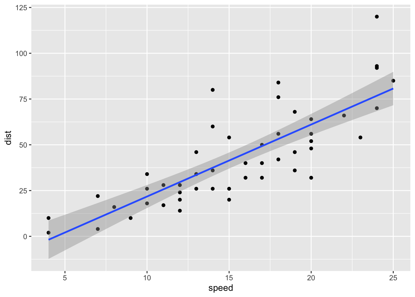
We can see that there are a few points on the graph that may be unduly influential. We’ll use a few more techniques to determine if we need to do something about these data points.
4.2 Leverage
Leverage values are useful for identifying abberant values, and we have a few ways to easily obtain and visualize these values in R. First, let’s create a new variable in our data frame that contains the leverage value for each observation. There’s not a hardfast cutoff to indicate if a leverage value is too high, so let’s calculate the median value and use that to see where the middle point is.
cars$lev <- hat(model.matrix(mod_a))
median(cars$lev)
## [1] 0.02945985We can then make a simple plot of these leverage values to see if any observations have a much larger value than the other observations. Based on our median lev value of 0.029, we can assume that values greatly above that may be unduly influential.
plot(cars$lev)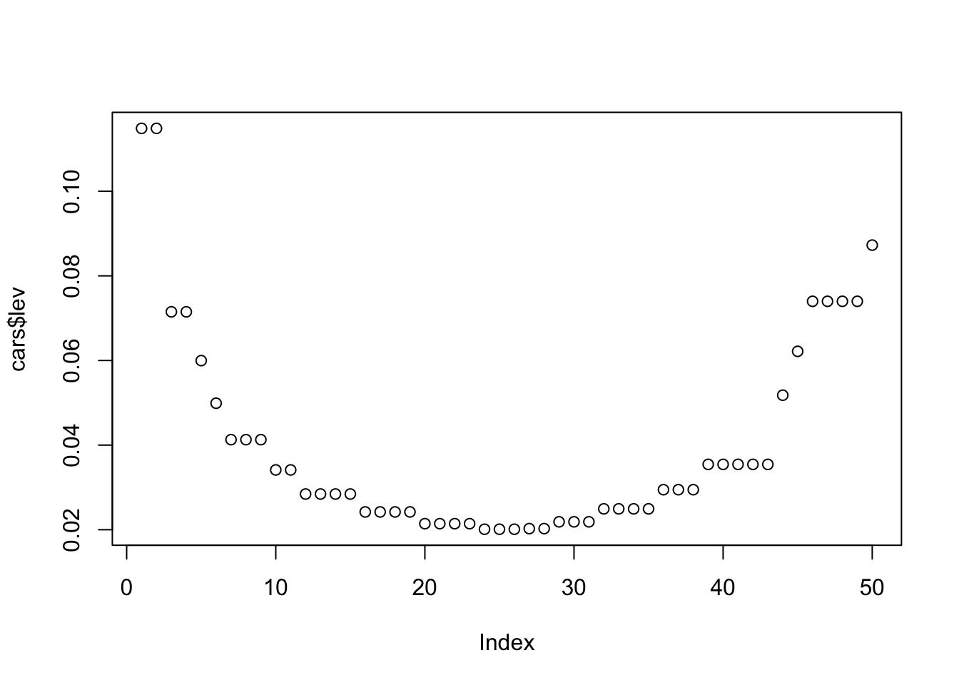
For this example, we’ll just arbitrarily choose 0.07 as our cutoff. Let’s take a peek at the observations that have greater leverage values than that.
ind <- which(cars$lev > 0.07)
cars[ind,]
## speed dist error_c sq_error_c x_diff pred_a error_a sq_error_a
## 1 4 2 -40.98 1679.3604 -11.4 -1.849460 3.849460 14.81834
## 2 4 10 -32.98 1087.6804 -11.4 -1.849460 11.849460 140.40970
## 3 7 4 -38.98 1519.4404 -8.4 9.947766 -5.947766 35.37593
## 4 7 22 -20.98 440.1604 -8.4 9.947766 12.052234 145.25633
## 46 24 70 27.02 730.0804 8.6 76.798715 -6.798715 46.22253
## 47 24 92 49.02 2402.9604 8.6 76.798715 15.201285 231.07906
## 48 24 93 50.02 2502.0004 8.6 76.798715 16.201285 262.48163
## 49 24 120 77.02 5932.0804 8.6 76.798715 43.201285 1866.35100
## 50 25 85 42.02 1765.6804 9.6 80.731124 4.268876 18.22330
## lev
## 1 0.11486131
## 2 0.11486131
## 3 0.07150365
## 4 0.07150365
## 46 0.07398540
## 47 0.07398540
## 48 0.07398540
## 49 0.07398540
## 50 0.087270074.3 Studentized Deleted Residuals
We can also use studentized deleted residuals to get an idea of influential observations in our data.
cars$stud_del_resid <- rstudent(mod_a)We can get a handy plot of these values with the ols_plot_resid_stud() function from the olsrr package.
ols_plot_resid_stud_fit(mod_a)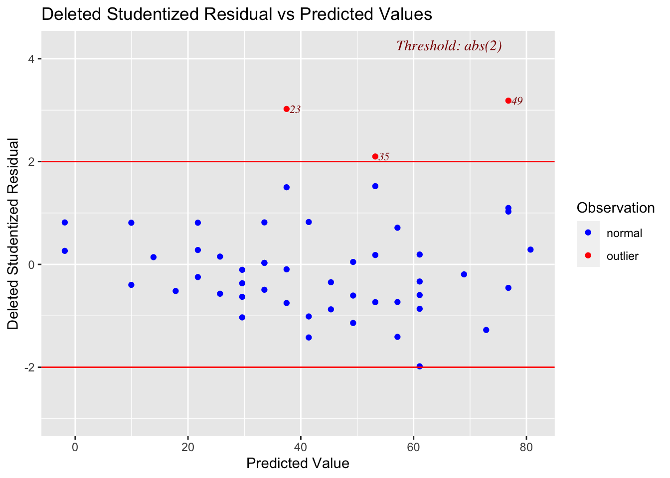
Notice that this plot gives the observation number for observations that are outside of its default diagnostic values.
4.3.1 Plot for leverage and studentized deleted residuals
The olsrr package also has a function that will plot your data by leverage and studentized deleted residuals. You want to pay special attention to any points that are indicated as being an outlier and having a high leverage value. Our plot below doesn’t show any values like that.
ols_plot_resid_lev(mod_a)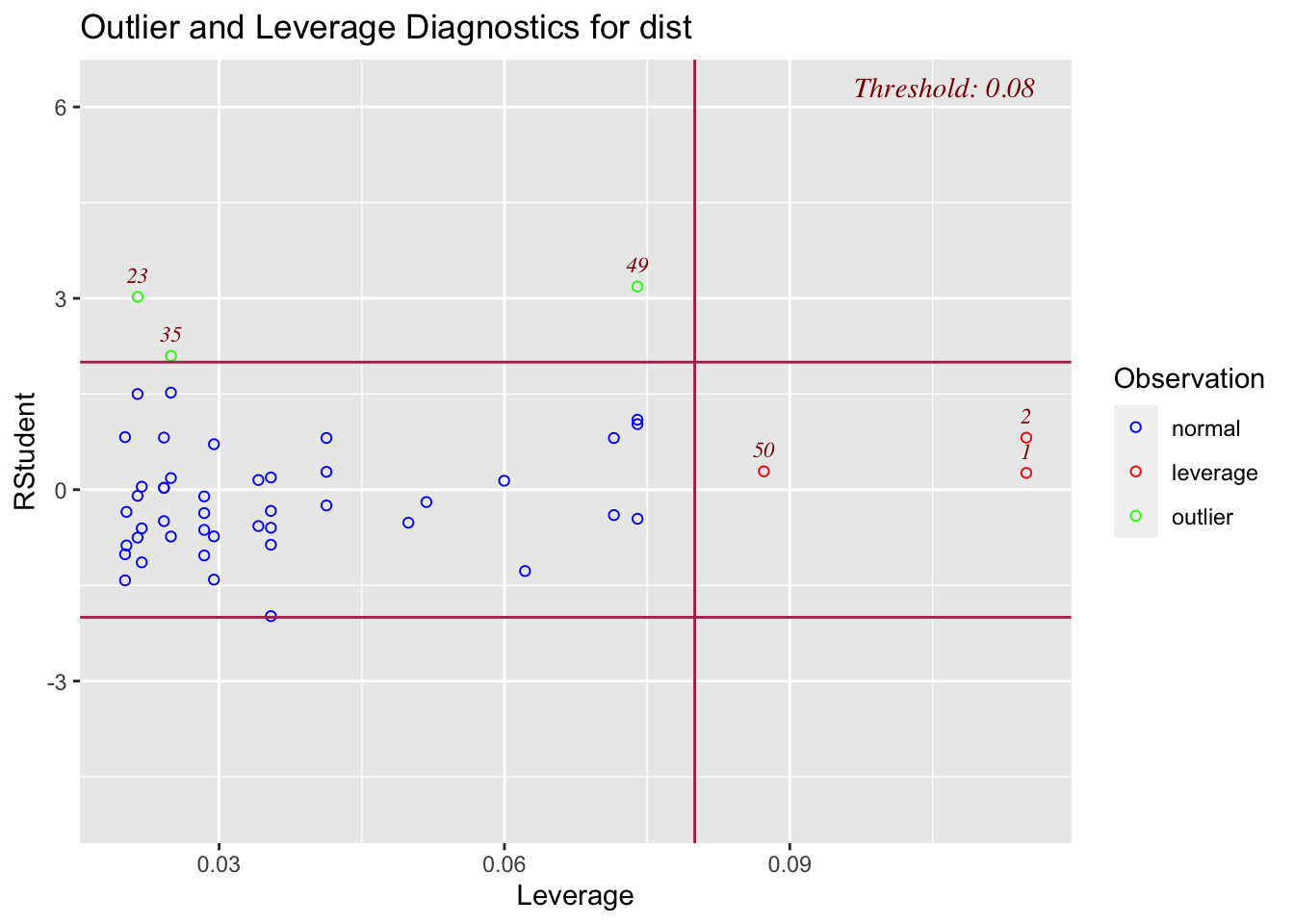
4.4 Cook’s Distance
Cook’s distance is another useful diagnostic that we can use. We can use these values similarly to how we used the previous diagnostics. The below graph will indicate the default diagnostic threshold and give the observation number for any observations that exceed that threshold.
ols_plot_cooksd_bar(mod_a)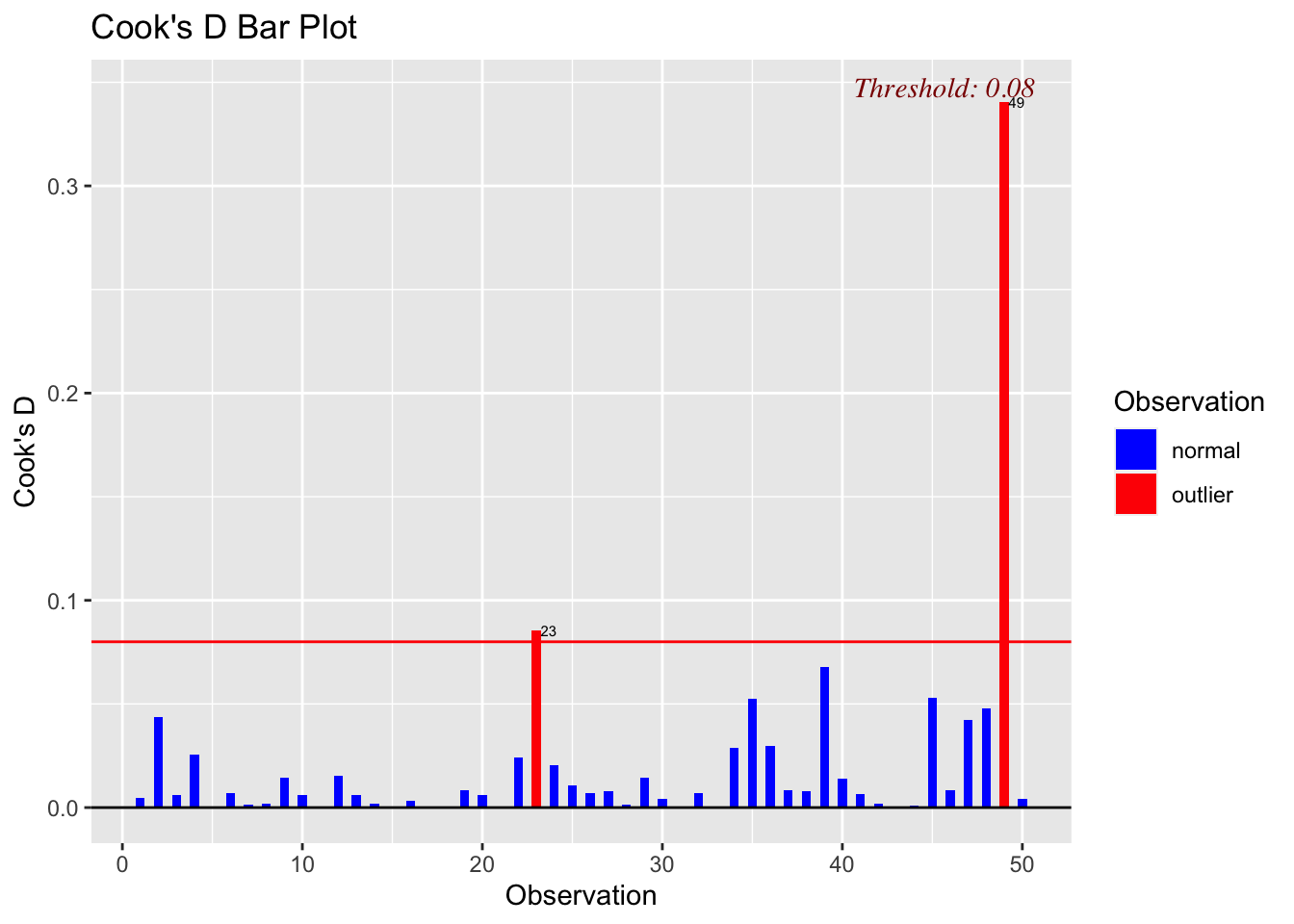
4.5 Non-Normal Error Distribution
It’s also a good idea to get an idea of the structure of your distriution of errors. We can do this easily by making a qq plot. Ideally you want the errors to fall on the line.
qqnorm(mod_a$residuals)
qqline(mod_a$residuals)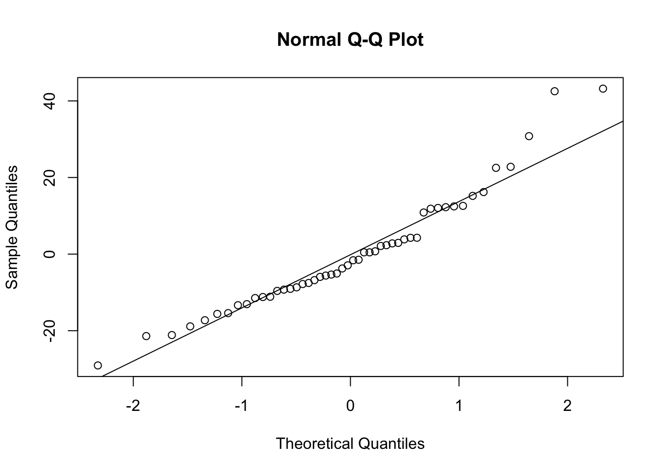
4.6 Homegeneity of Error Variance
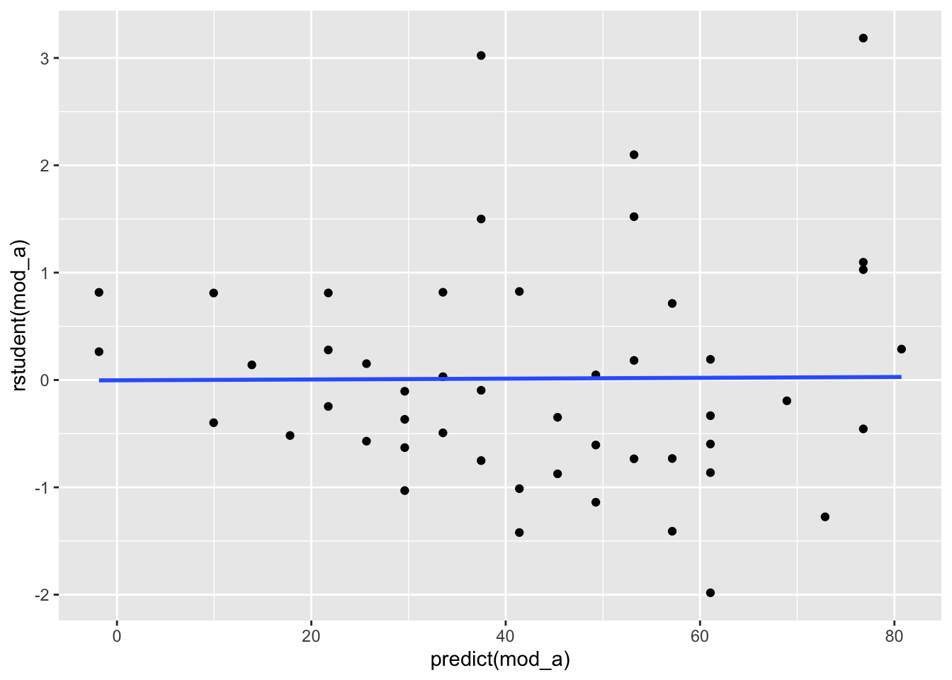
You also want to check that the error variances of your data are homogeneous. In the below plot, we would hope to see the residuals spread equally along the range of predictions. We don’t see this in the plot below; instead, we see a cone pattern that is typically indicative heteroscedasticity.
ggplot(data = cars, mapping = aes(x = predict(mod_a), y = rstudent(mod_a))) +
  geom_point() +
  geom_smooth(method = "lm", se = FALSE)