1 Overview

In this tutorial, we’ll cover how to perform a multiple regression analysis in R using the lm() function. We won’t go through the process step by step like we did in the Simple Linear Regression tutorial; however, you can use that tutorial as a guide for doing your multiple regression in a similar fashion. For this tutorial, we’ll be using the mtcars dataset available in R to predict the miles per gallon (mpg) of cars based on their weight (wt) and horsepower (hp).

1.1 Packages (and versions) used in this document

## [1] "R version 4.0.2 (2020-06-22)"
##  Package Version
##  ggplot2   3.3.2
##    olsrr   0.5.3

2 Simple Linear Regression

Before we get into the analyses, let’s take a quick peek at our data. This data frame has a number of variables that we won’t use in this tutorial, so I’ll go ahead and subset those out.

head(mtcars[,c(1,4,6)])
##                    mpg  hp    wt
## Mazda RX4         21.0 110 2.620
## Mazda RX4 Wag     21.0 110 2.875
## Datsun 710        22.8  93 2.320
## Hornet 4 Drive    21.4 110 3.215
## Hornet Sportabout 18.7 175 3.440
## Valiant           18.1 105 3.460

We’ll start off the analysis with a quick review of what was covered in the Simple Linear Regression tutorial. We’ll use the lm() function to create two single predictor models for predicting mpg. We’ll start off with using wt as our predictor.

wt_mod <- lm(mpg ~ wt, data = mtcars)
summary(wt_mod)
## 
## Call:
## lm(formula = mpg ~ wt, data = mtcars)
## 
## Residuals:
##     Min      1Q  Median      3Q     Max 
## -4.5432 -2.3647 -0.1252  1.4096  6.8727 
## 
## Coefficients:
##             Estimate Std. Error t value Pr(>|t|)    
## (Intercept)  37.2851     1.8776  19.858  < 2e-16 ***
## wt           -5.3445     0.5591  -9.559 1.29e-10 ***
## ---
## Signif. codes:  0 '***' 0.001 '**' 0.01 '*' 0.05 '.' 0.1 ' ' 1
## 
## Residual standard error: 3.046 on 30 degrees of freedom
## Multiple R-squared:  0.7528, Adjusted R-squared:  0.7446 
## F-statistic: 91.38 on 1 and 30 DF,  p-value: 1.294e-10

And now we’ll try hp as our predictor.

hp_mod <- lm(mpg ~ hp, data = mtcars)
summary(hp_mod)
## 
## Call:
## lm(formula = mpg ~ hp, data = mtcars)
## 
## Residuals:
##     Min      1Q  Median      3Q     Max 
## -5.7121 -2.1122 -0.8854  1.5819  8.2360 
## 
## Coefficients:
##             Estimate Std. Error t value Pr(>|t|)    
## (Intercept) 30.09886    1.63392  18.421  < 2e-16 ***
## hp          -0.06823    0.01012  -6.742 1.79e-07 ***
## ---
## Signif. codes:  0 '***' 0.001 '**' 0.01 '*' 0.05 '.' 0.1 ' ' 1
## 
## Residual standard error: 3.863 on 30 degrees of freedom
## Multiple R-squared:  0.6024, Adjusted R-squared:  0.5892 
## F-statistic: 45.46 on 1 and 30 DF,  p-value: 1.788e-07

We can see from the summaries of these models, that both wt and hp were significant individual predictors of mpg at the p<.001 level. But you came to this tutorial to learn about multiple regression, not Simple Linear Regression.

3 Multiple Regression

In this section, we’ll look at an easy way to specify additional predictors in your regression model.

3.1 Main Effects

The lm() function makes adding additional predictors to our regression formulas incredibly easy. We can simply just add the predictor (pun intended) to our model, as shown below.

wthp_mod <- lm(mpg ~ wt + hp, data = mtcars)
summary(wthp_mod)
## 
## Call:
## lm(formula = mpg ~ wt + hp, data = mtcars)
## 
## Residuals:
##    Min     1Q Median     3Q    Max 
## -3.941 -1.600 -0.182  1.050  5.854 
## 
## Coefficients:
##             Estimate Std. Error t value Pr(>|t|)    
## (Intercept) 37.22727    1.59879  23.285  < 2e-16 ***
## wt          -3.87783    0.63273  -6.129 1.12e-06 ***
## hp          -0.03177    0.00903  -3.519  0.00145 ** 
## ---
## Signif. codes:  0 '***' 0.001 '**' 0.01 '*' 0.05 '.' 0.1 ' ' 1
## 
## Residual standard error: 2.593 on 29 degrees of freedom
## Multiple R-squared:  0.8268, Adjusted R-squared:  0.8148 
## F-statistic: 69.21 on 2 and 29 DF,  p-value: 9.109e-12

We can see from the summary above that this model includes both wt and hp as predictors in our model. We can also see that the reported t-values (and their respective p-values) for each predictor have changed, as we might expect from having multiple predictors in the model.

We may wish to run a simple model comparison to see if the trade-off between the added complexity of our additional terms and the increase in PRE (Proportional Reduction in Error; Multiple R-squared) is worth it. We can do this with the anova() function.

anova(wt_mod, hp_mod, wthp_mod)
## Analysis of Variance Table
## 
## Model 1: mpg ~ wt
## Model 2: mpg ~ hp
## Model 3: mpg ~ wt + hp
##   Res.Df    RSS Df Sum of Sq      F   Pr(>F)    
## 1     30 278.32                                 
## 2     30 447.67  0   -169.35                    
## 3     29 195.05  1    252.63 37.561 1.12e-06 ***
## ---
## Signif. codes:  0 '***' 0.001 '**' 0.01 '*' 0.05 '.' 0.1 ' ' 1

From this output, we can see that the model including both predictor main effects is a significant improvement over the single-term models.
3.2 Interaction Effects

If you’re curious about how to add interaction terms to your models, go check out the Moderated and Nonlinear Regression tutorial (after you finish this one, of course).

4 Diagnostics and Assumption Checking

We can use many of the same techniques that we saw in the Simple Linear Regression tutorial to run diagnostics on our multiple regression.

4.1 Leverage

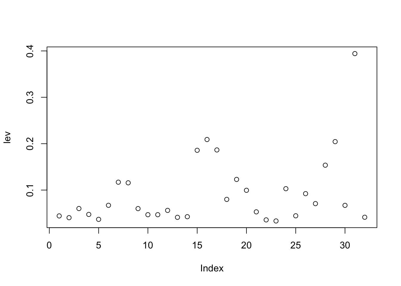
Leverage values are useful for identifying abberant values, and we have a few ways to easily obtain and visualize these values in R. First, let’s create a new variable in our data frame that contains the leverage value for each observation. There’s not a hardfast cutoff to indicate if a leverage value is too high, so let’s calculate the median value and use that to see where the middle point is.

lev <- hat(model.matrix(wthp_mod))
median(lev)
## [1] 0.06362374

We can then make a simple plot of these leverage values to see if any observations have a much larger value than the other observations. Based on our median lev value of 0.064, we can assume that values greatly above that may be unduly influential.

plot(lev)

For this example, we’ll just arbitrarily choose 0.15 as our cutoff. Let’s take a peek at the observations that have greater leverage values than that.

ind <- which(lev > 0.15)
mtcars[ind,]
##                      mpg cyl  disp  hp drat    wt  qsec vs am gear carb
## Cadillac Fleetwood  10.4   8 472.0 205 2.93 5.250 17.98  0  0    3    4
## Lincoln Continental 10.4   8 460.0 215 3.00 5.424 17.82  0  0    3    4
## Chrysler Imperial   14.7   8 440.0 230 3.23 5.345 17.42  0  0    3    4
## Lotus Europa        30.4   4  95.1 113 3.77 1.513 16.90  1  1    5    2
## Ford Pantera L      15.8   8 351.0 264 4.22 3.170 14.50  0  1    5    4
## Maserati Bora       15.0   8 301.0 335 3.54 3.570 14.60  0  1    5    8

4.2 Studentized Deleted Residuals

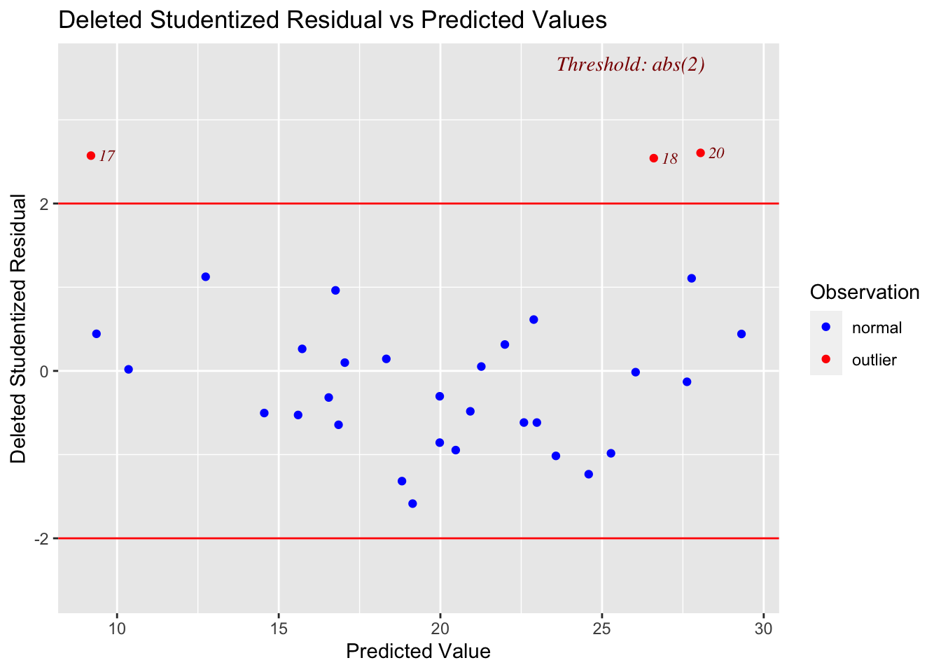
We can also use studentized deleted residuals to get an idea of influential observations in our data.

stud_del_resid <- rstudent(wthp_mod)

We can get a handy plot of these values with the ols_plot_resid_stud() function from the olsrr package.

ols_plot_resid_stud_fit(wthp_mod)

Notice that this plot gives the observation number for observations that are outside of its default diagnostic values.

4.2.1 Plot for leverage and studentized deleted residuals

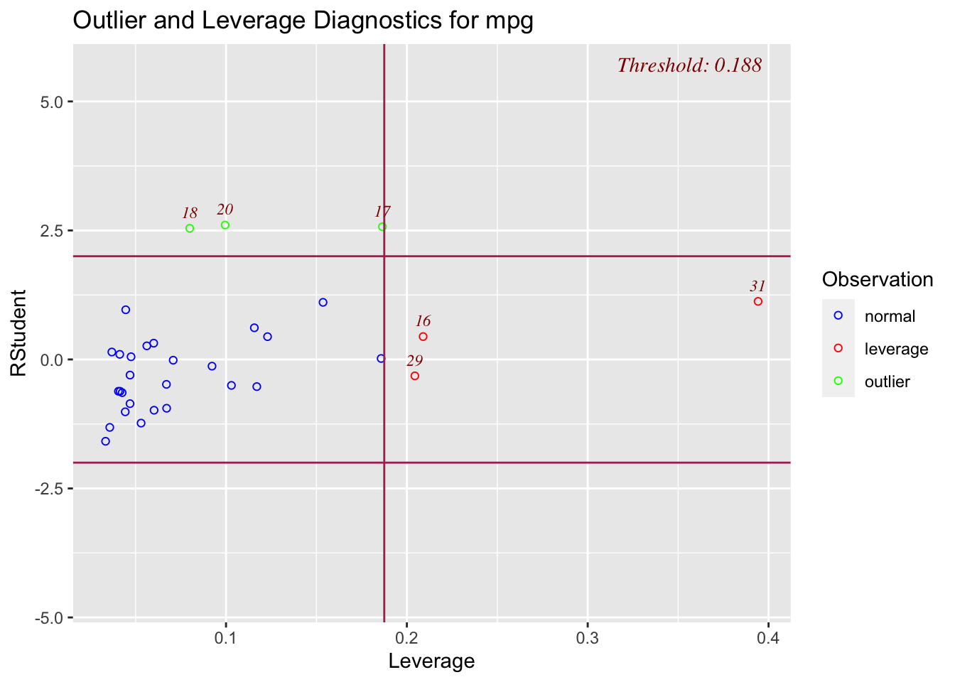
The olsrr package also has a function that will plot your data by leverage and studentized deleted residuals. You want to pay special attention to any points that are indicated as being an outlier and having a high leverage value. Our plot below doesn’t show any values like that, but observation 17 is pretty close.

ols_plot_resid_lev(wthp_mod)

4.3 Cook’s Distance

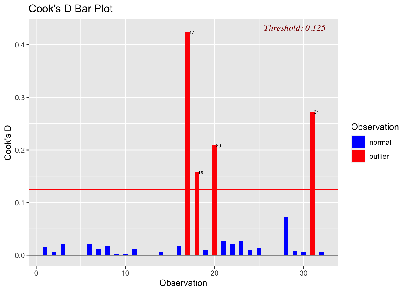
Cook’s distance is another useful diagnostic that we can use. We can use these values similarly to how we used the previous diagnostics. The below graph will indicate the default diagnostic threshold and give the observation number for any observations that exceed that threshold.

ols_plot_cooksd_bar(wthp_mod)

4.4 Non-Normal Error Distribution

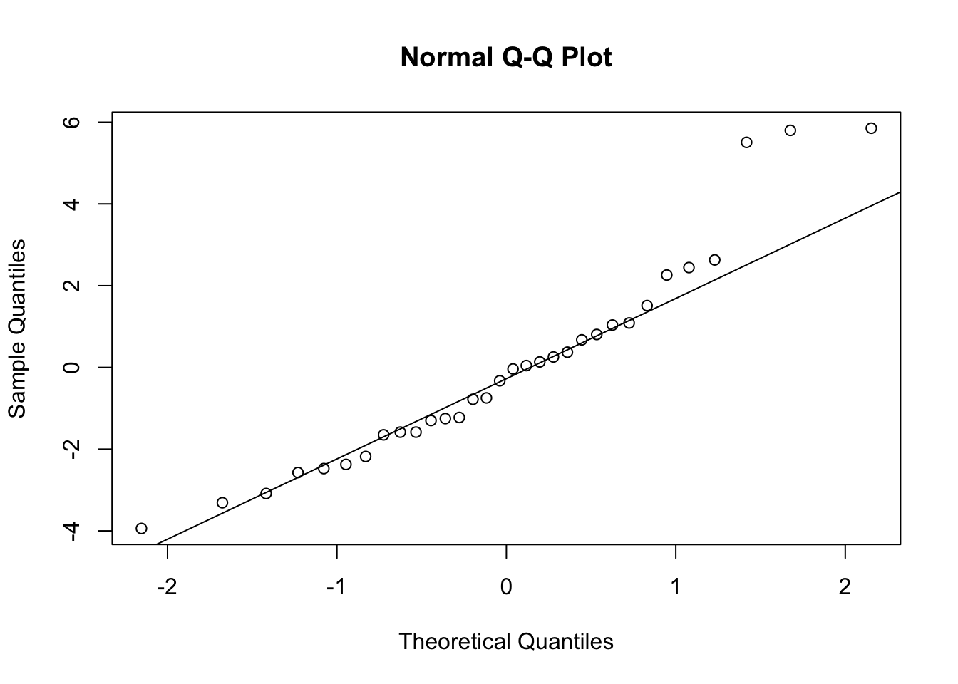
It’s also a good idea to get an idea of the structure of your distriution of errors. We can do this easily by making a qq plot. Ideally you want the errors to fall on the line.

qqnorm(wthp_mod$residuals)
qqline(wthp_mod$residuals)

4.5 Homegeneity of Error Variance

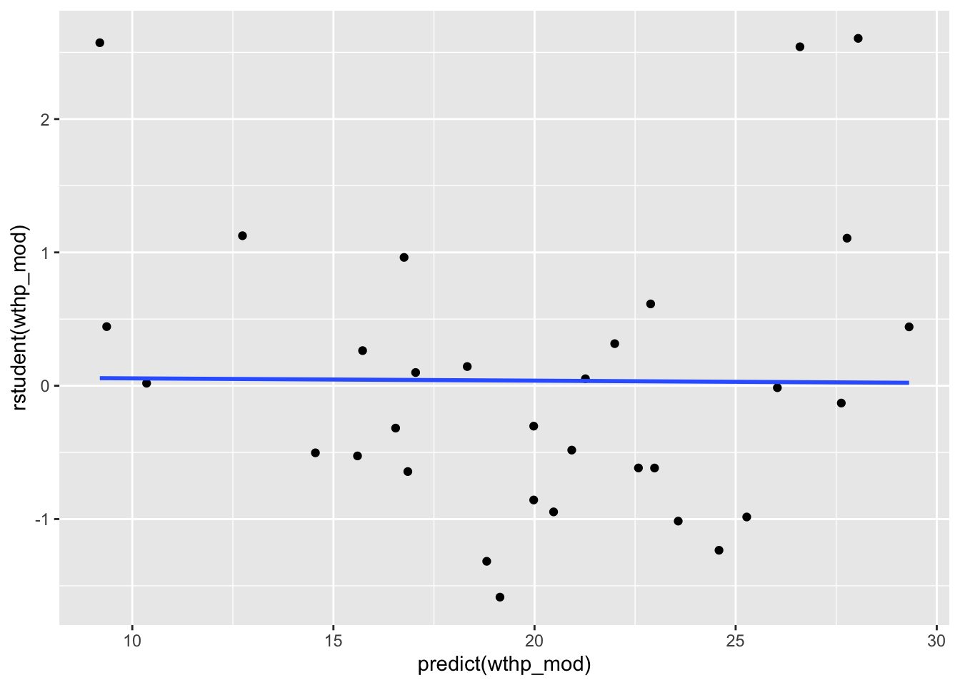
You also want to check that the error variances of your data are homogeneous. In the below plot, we would hope to see the residuals spread equally along the range of predictions. We don’t see this in the plot below; instead, we see sparser predictions below 15 and above 25 (most falling above the line) and denser predictions between 15 and 25 (a majority falling below the line).

ggplot(data = mtcars, mapping = aes(x = predict(wthp_mod), y = rstudent(wthp_mod))) +
  geom_point() +
  geom_smooth(method = "lm", se = FALSE)