- 1 Overview
- 1.1 Packages (and versions) used in this document
- 2 Two-way ANOVA
- 2.1 Getting Familiar with the Data
- 2.1.1 Descriptive Statistics
- 2.2 The Analysis
- 2.2.1 Brief Overview of SS Types
- 2.2.2 Performing the Two-Way ANOVA
- 2.3 Visualizing the Results
x-Way ANOVA
Original Author: Kyle R. Ripley
Updated on 6/25/2020 by Kyle R. Ripley
1 Overview
In this tutorial, we’ll build on the concepts discussed in the One-Way ANOVA tutorial. We’ll explicitly cover how to perform a two-way ANOVA, but the procedures shown here can be translated to three-way ANOVAs and so on. We’ll also cover the different types of sums of squares and how they affect the results of your ANOVA. For this tutorial, we’ll be using the mtcars dataset available in R to look at the differences in miles per gallon (mpg) of cars with different types of engines (vs) and transmission (am).
1.1 Packages (and versions) used in this document
## [1] "R version 4.0.2 (2020-06-22)"## Package Version
## dplyr 1.0.2
## car 3.0-9
## ggplot2 3.3.22 Two-way ANOVA
2.1 Getting Familiar with the Data
Before jumping into the analysis, let’s take a peek at our data. We’ll use str() to check the class of our variables, and we’ll use summary() to get an overview of our data frame - such as missingness, distribution information of variables, etc.
str(mtcars)## 'data.frame': 32 obs. of 11 variables:
## $ mpg : num 21 21 22.8 21.4 18.7 18.1 14.3 24.4 22.8 19.2 ...
## $ cyl : num 6 6 4 6 8 6 8 4 4 6 ...
## $ disp: num 160 160 108 258 360 ...
## $ hp : num 110 110 93 110 175 105 245 62 95 123 ...
## $ drat: num 3.9 3.9 3.85 3.08 3.15 2.76 3.21 3.69 3.92 3.92 ...
## $ wt : num 2.62 2.88 2.32 3.21 3.44 ...
## $ qsec: num 16.5 17 18.6 19.4 17 ...
## $ vs : num 0 0 1 1 0 1 0 1 1 1 ...
## $ am : num 1 1 1 0 0 0 0 0 0 0 ...
## $ gear: num 4 4 4 3 3 3 3 4 4 4 ...
## $ carb: num 4 4 1 1 2 1 4 2 2 4 ...From the str() output, we can see that our outcome variable (mpg) is of the numeric class, which it should be. However, we can see that vs and am are also numeric, but we want them to be factors. We’ll need to fix this.
mtcars$vs <- factor(mtcars$vs, levels = c(0, 1), labels = c("V-shaped", "straight"))
mtcars$am <- factor(mtcars$am, levels = c(0, 1), labels = c("automatic", "manual"))
str(mtcars)
## 'data.frame': 32 obs. of 11 variables:
## $ mpg : num 21 21 22.8 21.4 18.7 18.1 14.3 24.4 22.8 19.2 ...
## $ cyl : num 6 6 4 6 8 6 8 4 4 6 ...
## $ disp: num 160 160 108 258 360 ...
## $ hp : num 110 110 93 110 175 105 245 62 95 123 ...
## $ drat: num 3.9 3.9 3.85 3.08 3.15 2.76 3.21 3.69 3.92 3.92 ...
## $ wt : num 2.62 2.88 2.32 3.21 3.44 ...
## $ qsec: num 16.5 17 18.6 19.4 17 ...
## $ vs : Factor w/ 2 levels "V-shaped","straight": 1 1 2 2 1 2 1 2 2 2 ...
## $ am : Factor w/ 2 levels "automatic","manual": 2 2 2 1 1 1 1 1 1 1 ...
## $ gear: num 4 4 4 3 3 3 3 4 4 4 ...
## $ carb: num 4 4 1 1 2 1 4 2 2 4 ...That’s better. Now let’s move on to the summary() of our data.
summary(mtcars)## mpg cyl disp hp
## Min. :10.40 Min. :4.000 Min. : 71.1 Min. : 52.0
## 1st Qu.:15.43 1st Qu.:4.000 1st Qu.:120.8 1st Qu.: 96.5
## Median :19.20 Median :6.000 Median :196.3 Median :123.0
## Mean :20.09 Mean :6.188 Mean :230.7 Mean :146.7
## 3rd Qu.:22.80 3rd Qu.:8.000 3rd Qu.:326.0 3rd Qu.:180.0
## Max. :33.90 Max. :8.000 Max. :472.0 Max. :335.0
## drat wt qsec vs am
## Min. :2.760 Min. :1.513 Min. :14.50 V-shaped:18 automatic:19
## 1st Qu.:3.080 1st Qu.:2.581 1st Qu.:16.89 straight:14 manual :13
## Median :3.695 Median :3.325 Median :17.71
## Mean :3.597 Mean :3.217 Mean :17.85
## 3rd Qu.:3.920 3rd Qu.:3.610 3rd Qu.:18.90
## Max. :4.930 Max. :5.424 Max. :22.90
## gear carb
## Min. :3.000 Min. :1.000
## 1st Qu.:3.000 1st Qu.:2.000
## Median :4.000 Median :2.000
## Mean :3.688 Mean :2.812
## 3rd Qu.:4.000 3rd Qu.:4.000
## Max. :5.000 Max. :8.000From the summary() output, we can see that we don’t have equal sample sizes in each level of vs and am. We can also see some distributional information about the measurement variables.
2.1.1 Descriptive Statistics
It’ll also be helpful in reporting our results to have some idea of what our descriptive statistics are. We’ll retrieve them differently here than we did in the One-Way ANOVA tutorial. We’ll use the group_by() and summarise() functions from the dplyr package.
summarise(.data = group_by(mtcars, vs, am), mean = mean(mpg), sd = sd(mpg), n = n())## # A tibble: 4 x 5
## # Groups: vs [2]
## vs am mean sd n
## <fct> <fct> <dbl> <dbl> <int>
## 1 V-shaped automatic 15.0 2.77 12
## 2 V-shaped manual 19.8 4.01 6
## 3 straight automatic 20.7 2.47 7
## 4 straight manual 28.4 4.76 72.2 The Analysis
As discussed in the One-Way ANOVA tutorial, we could use either lm() or aov() for our ANOVAs, but I’ll be using lm() in this tutorial. Before we get into the actual analysis, we need to have a discussion about the different types of sums of squares.
2.2.1 Brief Overview of SS Types
Now that we’ll have more than one predictor variable, we need to be aware of the types of sums of squares and when they should be used.
2.2.1.1 Type I SS
Type I SS considers the predictors sequentially. This isn’t particularly useful for unbalanced studies (like the one we’re examining in this tutorial), but is useful for parsimonious quadratic models. The anova() function defaults to using Type I SS.
2.2.1.2 Type II SS
Type II SS adjusts the effects of a predictor (a) for an effect (b) if, and only if, (b) does not contain (a). For example:
In an A + B + A*B model, A would be adjusted for B, B would be adjusted for A, and A*B would be adjusted for A and B (because neither contains the term A*B).
If the model contains only main effects, then type II SS and type III SS will be the same.
2.2.1.3 Type III SS
For type III SS, every effect (predictor) is adjusted for all other effects. This allows a comparison of main effects in the presence of an interaction.
2.2.2 Performing the Two-Way ANOVA
Now that we know a bit about the types of SS, we can go ahead and conduct our two-way ANOVA. We’ll also use this as an opportunity to illustrate what was said in the previous section about SS. We’ll go ahead an specify two different models - one with transmission type before engine type, and the other reversed.
m1 <- lm(mpg ~ am + vs, data = mtcars)
m2 <- lm(mpg ~ vs + am, data = mtcars)
Below you’ll see the anova() output for m1.
anova(m1)## Analysis of Variance Table
##
## Response: mpg
## Df Sum Sq Mean Sq F value Pr(>F)
## am 1 405.15 405.15 33.239 3.038e-06 ***
## vs 1 367.41 367.41 30.142 6.501e-06 ***
## Residuals 29 353.49 12.19
## ---
## Signif. codes: 0 '***' 0.001 '**' 0.01 '*' 0.05 '.' 0.1 ' ' 1And now we’ll take a look at the anova() output for m2. Remember that our two-way ANOVA is unbalanced (different n in each group), and anova() defaults to type I SS. Because of this, we’ll have different estimates in our models even though they have the same predictors.
anova(m2)## Analysis of Variance Table
##
## Response: mpg
## Df Sum Sq Mean Sq F value Pr(>F)
## vs 1 496.53 496.53 40.735 5.610e-07 ***
## am 1 276.03 276.03 22.646 4.958e-05 ***
## Residuals 29 353.49 12.19
## ---
## Signif. codes: 0 '***' 0.001 '**' 0.01 '*' 0.05 '.' 0.1 ' ' 1Because of this, we should opt to use a different type of SS. We can’t do this with the anova() function, we’ll turn to the Anova() (capital A) function from the car package. With this function, we can specify whether we want to use type II SS or type III SS. Below, we’ll look at type II SS for both models.
Anova(m1, type = 2)## Anova Table (Type II tests)
##
## Response: mpg
## Sum Sq Df F value Pr(>F)
## am 276.03 1 22.646 4.958e-05 ***
## vs 367.41 1 30.142 6.501e-06 ***
## Residuals 353.49 29
## ---
## Signif. codes: 0 '***' 0.001 '**' 0.01 '*' 0.05 '.' 0.1 ' ' 1Notice that we get the same estimates for both models (just in a different order) when we use type II SS.
Anova(m2, type = 2)## Anova Table (Type II tests)
##
## Response: mpg
## Sum Sq Df F value Pr(>F)
## vs 367.41 1 30.142 6.501e-06 ***
## am 276.03 1 22.646 4.958e-05 ***
## Residuals 353.49 29
## ---
## Signif. codes: 0 '***' 0.001 '**' 0.01 '*' 0.05 '.' 0.1 ' ' 1Because our model only includes main effects (no interactions), we could also opt to use type III SS, and we’d get the same result, as shown below. Notice that the type III SS option also includes the intercept values.
Anova(m1, type = 3)## Anova Table (Type III tests)
##
## Response: mpg
## Sum Sq Df F value Pr(>F)
## (Intercept) 3026.81 1 248.320 9.352e-16 ***
## am 276.03 1 22.646 4.958e-05 ***
## vs 367.41 1 30.142 6.501e-06 ***
## Residuals 353.49 29
## ---
## Signif. codes: 0 '***' 0.001 '**' 0.01 '*' 0.05 '.' 0.1 ' ' 12.3 Visualizing the Results
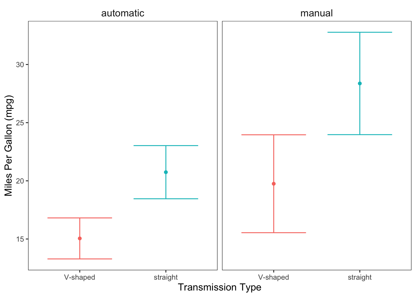
Now that we’ve seen that mpg is significantly different for levels of am and vs, we may want to visualize this relationship. This is easy to do if you’re familiar with Graphing in ggplot2.
ggplot(data = mtcars, mapping = aes(x = am, y = mpg, color = am)) +
  geom_point(stat = "summary", fun = "mean") +
  geom_errorbar(stat = "summary", fun.data = "mean_cl_normal", width = 0.75) +
  facet_wrap(facets = ~ vs) +
  labs(x = "Transmission Type", y = "Miles Per Gallon (mpg)") +
  jtools::theme_apa(legend.pos = "none")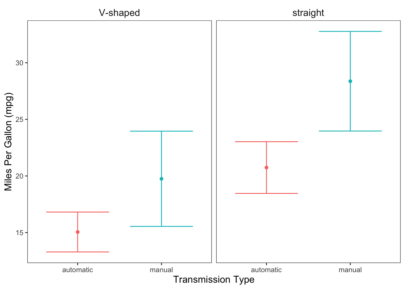
ggplot(data = mtcars, mapping = aes(x = vs, y = mpg, color = vs)) +
  geom_point(stat = "summary", fun = "mean") +
  geom_errorbar(stat = "summary", fun.data = "mean_cl_normal", width = 0.75) +
  facet_wrap(facets = ~ am) +
  labs(x = "Transmission Type", y = "Miles Per Gallon (mpg)") +
  jtools::theme_apa(legend.pos = "none")